Note: this post is about You Have Type 1 and is a continuation of Part I.

You Have Type 1 is a really good learning experience for me, too. In addition to web development (I’m using Flask and sqlite on the backend, and d3 on the frontend to build plots), it’s a good software engineering exercise.

I get to do a bit of data, too.

One thing that I really want to do is personalize the simulator. I want the user to really feel like they have type 1 (the game is called “You Have Type 1” after all!). So to do that, I need to fit the model that I’m using to simulate the game to the player.

This is not really a trivial task. The simulator parameters are avaialable in a file called vpatientparams.csv that has like 60 columns, each with some very specific model parameters (as a sample, here are some: 'x0_ 1', 'x0_ 2', 'kabs', 'kmax', 'kmin', 'b', 'd', 'Vg', 'Vi'… et cetera). These do correspond to real physical things in the body – the simulation is a pharmacokinetic “container” model, with containers for the stomach, plasma, etc. But I do not really know how any of this stuff works. It’s interesting, but I’m really on a broader mission here.

Unfortunately, the people who use my game do not know their own Vi or x0_ 2 parameter, so they can’t just give me theirs so I can personalize the simulator. One parameter that people do know about themselves is their body weight. So I can ask for their body weight, and then infer the parameters based on that.

Now: please keep in mind. People are not going to use You Have Type 1 to make clinical decisions about their Type 1. That is NOT the intention of the app. So, I don’t need a PhD level of accuracy for inferring these parameters. I just need some customization that is “close enough” to make gameplay more compelling to people who are not diabetics. If anyone reading this post has any suggestions as to how I could improve personalization, please let me know! I want to do it right!

Gaussian Process Regression

With all that said, here’s how I am going to do this. I’m going to assume that these parameters are stationary with regard to body weight, and that they are iid variables. With these assumptions in mind (and I’m SURE – they are very very broad and simple assumptions!) I’m going to fit a model for each parameter to predict how it varies with body weight.

So what I’m going to do is use gaussian_process from sklearn to train my model.

I have 30 patients – 10 adults, 10 children, and 10 adolescents. I’m going to train a model to approximate the function \( f(w) \) which maps the body weight to the parameter in question. I think the structure of a gaussian process forbids me from mixing categorical (“adult” “child” “adolescent”) with continuous data (“body weight”). So: let’s say my player is an adult. For each parameters, I will build a model that uses the 10 data points from that parameter to create a regression. I’ll do this for each parameter, and for each age group. So, in the end, I will have \( 10 \text{patients} \times 50 \text{parameters} \times 3 \text{age groups} \) which is 1500 data points split between 150 different models, 10 data points for each model.

This is not bad, but not great either. See my disclaimer above.

A good overview of gaussian process regression can be found in Gaussian Processes for Machine Learning, by Carl Edward Rasmussen and Christopher K. I. Williams – it’s available for free online at that link. Quite math heavy. Since I already read a lot of the Rasmussen book and I haven’t touched GPR for a couple years, I looked at Quick Start to Gaussian Process Regression on Towards Data Science for a quicker sklearn.gaussian_process tutorial. The gaussian_process api is quite intuitive and easy to follow with a bit of background on GPR.

What we do is load the data into pandas and create the necessary objects for fitting:

    import sklearn.gaussian_process as gp
    import pandas as pd

    data = pd.read_csv("./vpatient_params.csv")

    """Here, I pruned the columns in `data` that had a bunch of identical values"""

    for c in chart:
        kernel = (
            gp.kernels.ConstantKernel()
            + gp.kernels.ConstantKernel()
            * gp.kernels.RBF(length_scale=10, length_scale_bounds="fixed")
            + gp.kernels.WhiteKernel()
        )
        gpr = gp.GaussianProcessRegressor(kernel=kernel, n_restarts_optimizer=n_retries)
        X, y = data["BW"].values.reshape(-1, 1), data[c].values.reshape(-1, 1)
        args.append(
            {
                "kernel": kernel,
                "gp": gpr,
                "x": X,
                "y": y,
                "c": c,
            }
        )
    return args, data, chart

The reason I packed all the ouputs into a list of args is that we can fit all our models in parallel, since they are independent of one another. I have 32 cores on my machine so this shortens fit time considerably!

There’s a few things that are notable here. The most important thing is the kernel that I made. Getting the kernel of a GPR model right is a bit of an art. In addition to compute time, kernels are one of the big drawbacks (or advantages, depending on how you look at it!) of GPR. Essentially, what the kernel is is a metric that tells you how close one data point \(x_i\) is from another \(x_j \) in the function space.

The Art of Kernel Design

So my kernel (also called a “Covariance Function”) looks something like this:

\( k(x_i, x_j) = C_1 -C_2 \exp( -|| x_i - x_j || ^2 / 2L^2) + C_3 \delta (x_i, x_j)\)

This kernel basically corresponds to some constant offset from zero \( C_1 \), plus an RBF relationship between the points \( -C_2 \exp( -|| x_i - x_j || ^2 / 2L^2) \), plus a bit of noise \( C_3 \delta (x_i, x_j)\)

Three RBF kernels with different “length” \(L\) parameters are shown above.You can see that when \(x=0\) and \(x=0\) are exactly equal, the kernel output is 1, which means that those two \(f(x)\) are exactly equal. If you compare \(x=0\) to \(x=10\), changing the length scale has a strong effect: at \(L=1\), those two points are not related at all (the output of the kernel is 0 at \(x=10\)), whereas if we increase the length scale to \(L=12\), \(x=10\) has a strong effect on the value of \(x=0\), and vice-versa! The shape of this curve tells us how the relationship between two points \(x_i\) and \(x_j\) changes in \(f(x)\) space as the difference between them grows and diminishes. And, another thing that is important about the RBF kernel in particular is that it is symmetric (\(x_i\) and \(x_j\) can swap places, and that does not change the relationship). Lastly, the kernel is “stationary,” which means that it doesn’t matter what \(x_i\) is: if there is another \(x_j\) that is the same distance away, difference in \(f(x)\) is the same.

So what we are saying, before even knowing anything about the data, is that the data points are all offset from zero by some amount \( C_1 \); they are related by a scaled RBF relationship in \(f(x)\) space by an RBF relationship, which is itself scaled by a parameter \(C_2\); and two identical points \(x_i\) and \(x_j\) have some noise (this is the \(\delta\) function).

What we are doing when we fit a GPR model is determining the values of these \(C_1, C_2, C_3\) parameters for each pair of data points \(x \) and \(f(x)\). This will then give us the basis upon which to draw new \(x\) points from the user, and then infer, based on the \(f(x)\) that we learned from fitting, what the parameter will be. For example, if we want the u2ss parameter, we make the assumption that it is a function of weight. Then weight is our \(x\) and u2ss is our \(f(x)\); we have 10 pairs of weight and u2ss. So we use the 10 pairs we know to fit the parameters of our kernel function \(C_1, C_2, C_3\), and subsequently when we get a new weight from the player of the game, \(x^\), we can ask our model and it will give us \(f(x^)\) that it learned.

Now, I’m going to make another kind of critical assumption, which is that I’m going to set the “length scale” hyperparameter in advance. I’m going to make a guess that for most of these parameters (u2ss, x_ 5 and so on), the params will be very very different between two people, if those people’s body weight is very very different. How different is very different? Well, I’m just going to choose it: 10kg. For the americans out there: 10kg is 22 pounds. What does this mean? If I have two data points, x=50kg and x=200kg, if I try to infer a parameter from a new data point \(x^=100\)kg, the model that I fit will not give me anything – because \(x^\) is way more than 10kg away from my other two data points. This assumption “seems right” to me. So I could be off. If I had a better background in pharmacokinetics I could more carefully set this parameter, or I could even vary it between patients. I’m not totally set on \(L=10\); it might be 30 or 50. But it’s definitely not \(L=1\); person A, who weighs 1kg more than person B, doesn’t have completely different pharmacokinetic properties from person B. But person C, who weighs 100kg more than person A and B, probably does. So we’ll just guess \(L\) to be in the range 10-30kg, and let the model learn \(L\), too.

This is what I mean by kernel design being kind of an art: we’ve made a bunch of a-priori assumptions about the data in order to design the kernel, and we’ve designed the kernel before even fitting the model! We don’t need to make these types of assumptions before e.g. fitting a neural network – that’s why GPR is limited in some ways. But then again, we can make some assumptions before fitting, which gives us a bit of power as long as we can make the right assumptions!

For more information about kernels, see: Gaussian Process Kernels on Towards Data Science, or the Kernel Cookbook by David Duvenaud.

Model Fit and Results

Alright, that’s the hard part. Now, we train. We’ll define a fit function that takes a single argument: arg, unpacks arg into the training data arrays x and y, and fit the model arg["gp"]. Then we return the fitted model, along with the parameter name arg["c"].

def fitfn(arg: dict) -> None:
    """function to fit model from args"""
    # check args
    for key in arg:
        if key not in {"kernel", "gp", "x", "y", "c"}:
            raise ValueError
    # fit the model
    arg["gp"].fit(arg["x"], arg["y"])
    # return the model
    return arg["c"], arg["gp"]

This is really kind of ugly code, but we only need to do it once, and we only have 1500 data points.

We can then use python’s great multiprocessing module to fit all of our parameters in parallel. I’m going to do this for all 30 patients (adults, children, and adolescents) at once, just to see what my outputs are. So here, we have a big list of args, which are themselves each dictionaries. For each arg in the list, we’ll pass it into fitfn. Once fitfn is done, we put the column (arg["c"]) and the fitted model (arg["gp"]) into a list. That list is called models and when pool.map is done, it is full of column names "c"’s, and models – the output of each fitfn call.

from multiprocessing import Pool

N_RETRIES = 6
args, data, chart = load_data(N_RETRIES)
pool = Pool()
models = pool.map(fitfn, args)

All we need to do from here is have a look at our fit models.

We define one more function, assess that will draw a plot of each one.

def assess(data: pd.DataFrame, chart: list, gps: list):
    """assess each model"""
    for c in chart:
        if c not in data.columns:
            raise ValueError

    # predict
    bws = np.linspace(data["BW"].min(), data["BW"].max(), num=200).reshape(-1, 1)

    gps_dict = {}
    for c, gp in gps:
        gps_dict[c] = gp

    figs, axs = [], []

    for k, (c, gpr) in enumerate(gps_dict.items()):

        if k % 6 == 0:
            if k != 0:
                # put existing into the list
                figs.append(fig)
                axs.append(ax)
            # reassign to new fig
            fig, ax = plt.subplots(nrows=2, ncols=3, figsize=(3, 2))

        j = k % 3
        i = k % 2

        yp, stdp = gpr.predict(bws, return_std=True)
        yp = np.squeeze(yp)
        ax[i, j].fill_between(np.squeeze(bws), yp - stdp, yp + stdp, alpha=0.1)
        ax[i, j].plot(np.squeeze(bws), yp)
        ax[i, j].scatter(data["BW"].values, data[c].values, label="c", s=MSIZE, c="k")
        ax[i, j].set_title(c)

    return figs, axs

Here, we’re going to sanity check that every column in chart exists in data; then we’re going to get a bunch of body weights that are within the range we have (that’s what the linspace function is doing). Then we’re going to unpack the list of tuples that are returned by each call of fitfn into a dict of models (gps_dict). So for each column in chart, we can retrieve the fitted model. This is obviously very lazy and not elegant at all but it works and hey we’re just exploring here!

Once we have that list, we just need to plot. Now, for each "BW", c pair (remember: "BW" is \(x\) and c is \(f(x)\)!) we are going to plot:

• The variance \(\sigma\) of c against a bunch of "BW" values, as a continuous shaded region;
• The inferrred c values against a bunch of "BW" values, as a continous line;
• The real c values against the real "BW" values (from the trainind data), as a scatter plot.

Since we have 50 parameters, we’re going to do this on several figures, each containing 6 plots. So figs is a list of figures and axs is a 2x3 array of ax once this loop is finished.

Let’s see those results!

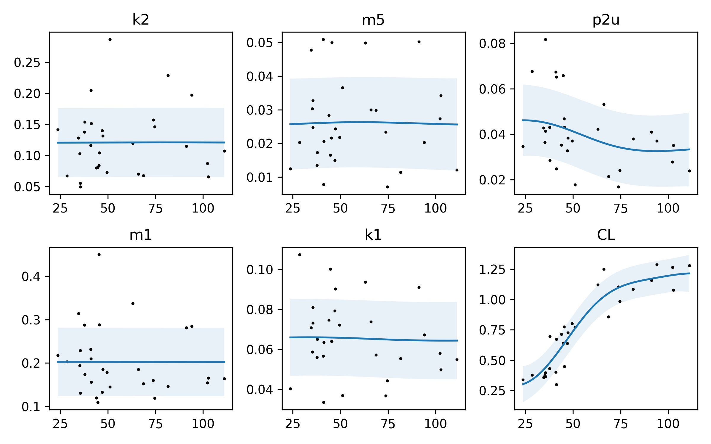
Here’s one plot. I should note, again: I don’t know what these parameters are, or what they mean! However, I can look at their relationship with bodyweight through these plots. Let’s remember what we’re looking at. The x-axis is body weight ^†, so we are plotting the value of each parameter against body weight. There’s kind of an interesting relationship with the parameters p2u and CL – they actually do vary with body weight. It looks like as body weight goes up, CL goes up. If I had to guess, I would say that p2u is related to an insulin sensitivity parameter, and CL is probably inversely related. Reading the paper again, we spot the p2u parameter (about a quarter of the way through the page, just below Figure 1). It looks like this parameter is related to the rate of insulin action on glucose utilization. If you’re familiar with Type 1, this may make sense: if you are a larger person, it takes a bit more time for insulin to get circulated around your body. That’s my guess as to what’s going on here. The others don’t vary that much, so maybe they are closer to pharmacokinetic “constants” that don’t vary much between people of differnet weights. Or it may be that the sample size is too small and the variance too high to really know.

There is also a lot of noise in our data – this is pretty well captured by the shaded region.

Let’s look at a few other plots:

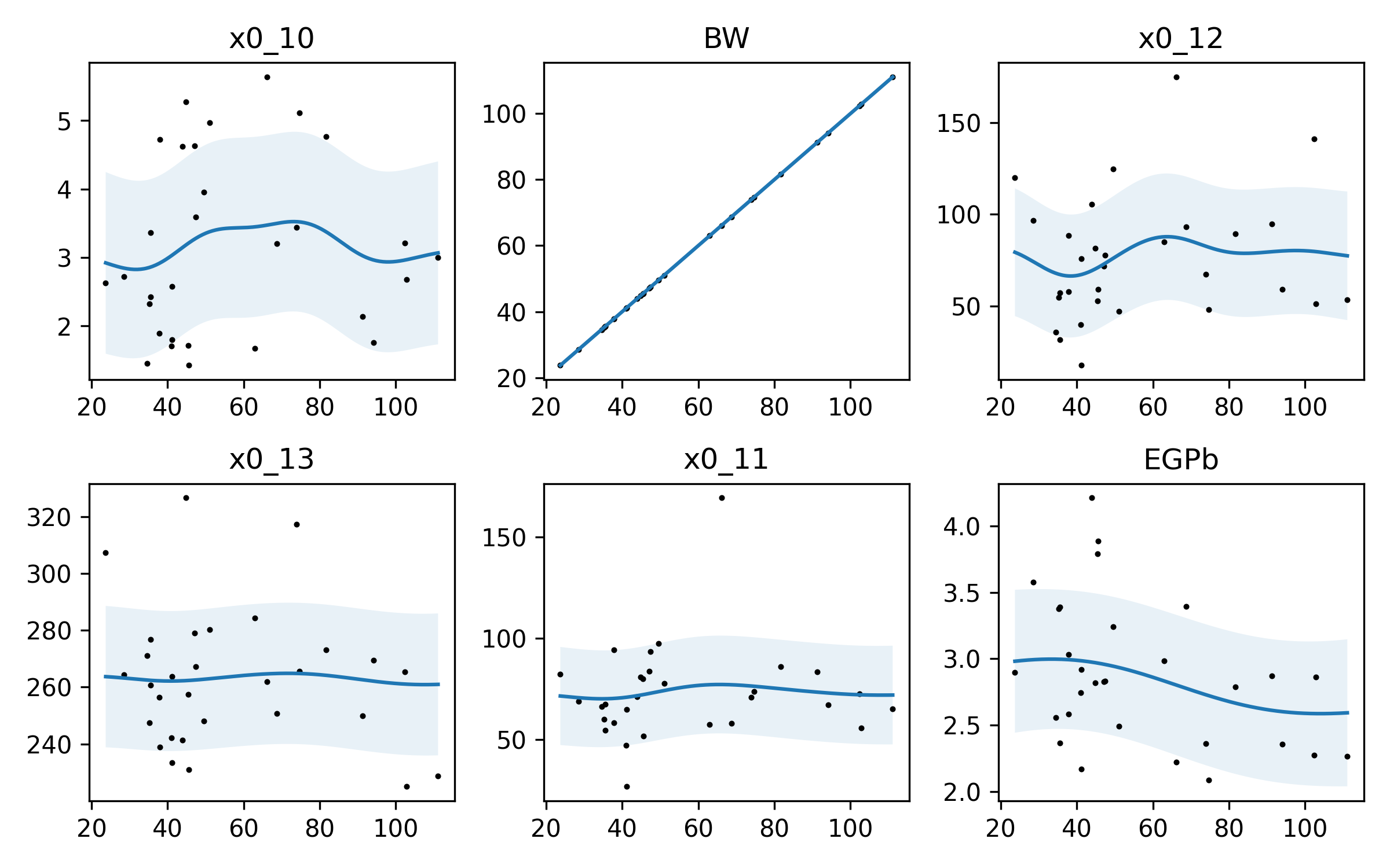
So here, again, we have some variablility. Now, GPR is not perfect. I think the squiggle in x0_10 is probably not quite that squiggly – we’re probably overfitting a bit.

And we can see another thing: the BW parameter is VERY accurately modeled. Why? BW is body weight, which is our independent variable. If you plot BW against BW, it’s a straight line: \(f(x) = x\)! Our model has learned that quite well!

Conclusions

So that’s it for now. I think GPR is well suited to the task of inferring our model parameters. Putting these parameters in and playing with the simulator will help, because there is a major unknown unknown here:

The Big Drawback

I have made the assumption here that all of these paramters are functions of body weight AND that their functional relationship with body weight is INDEPENDENT of their functional relationships with one another. This is a CRUCIAL assumption to make, and it may be our downfall, because the data is so variable!

Let’s look back at the very last figure above. We can see a sort of inverse “S” curve in EGPb. We may guess that EGPb decreases a bit when body weight increases. But this model tells us NOTHING about how EGPb relates to x0_11, or x0_10! If we chose randomly a value of EGPb from the distribution we have, that may strongly affect the value of x0_11. We have only inferred how these parameters relate to body weight, not how they relate to one another.

If we have more data (like the 300 patient commercial version of the simulator) we could gain a better understanding of these parameters by splitting the dataset into train/test parts and testing our predictions. All we’ve done here is assumed that these are independent processes governed by body weight!

But, it may be enough. We’ll test the actual simulation against a variety of body weights; overall, I expect insulin action to be quicker when body weight goes down. I expect correction factor (that is, the amount of insulin required to change the blood glucose) to go down as body weight goes up – when you are heavy, it takes more insulin to change your BG. And I expect that as weight increases, we will need more basal insulin to counteract the background tendency for the BG to rise.

Lastly, IF I am totally wrong, and I should have done this very differently, and a pharmacokinetics/biostatistician wants to step in to prevent my spreading misinformation, I will update this post – and update or abandon my approach to customizing the model. This is a game I’m making here, not an artificial pancreas, people!

UPDATE

It didn’t work. I think the critical mistake I made is that this actually isn’t a gaussian process. Which is the cause for dramatic failure when I apply Gaussian Process Regression to determine these parameters.

Now, I sort of knew this would happen at the outset, because this is a very finely tuned set of differential equations, and there’s no indication to my mathematical mind that two separate parameters in the governing equation would be jointly gaussian. It’s far more likely that each parameter interacts with the others in very specific and peculiar ways.

Ways that my “inferred” parameters failed:

• Glucose would trend up and up and up, no matter how much insulin was dosed – basal or bolus.
• Glucose would hardly respond to insulin or carbs – give 20u of insulin or eat 100g of carb, and the basal response dominates.
• Glucose would have a tremendous “momentum” – just a little bit of insulin or carb at the beginning would set it on a track to go up or down, without being able to stop it.

For a couple of randomly sampled models, I was able to get something approaching a “standard” glucose response. But all of the generated models were physically impossible; nobody is taking 500u of insulin in one day.

Now, I mentioned that this was an FDA-approved simulator that they use to test artificial pancreas algorithms in-silico. That means that these artificial patients – my original dataset – are not actually real people. They’re actually “edge cases,” that are designed to be just at the very edge of the distribution of real people with regards to these model parameters. This is because if a researcher tests an artificial pancreas (AP) model on the simulator, and it works against all of these challenging “edge cases,” it is very likely to work on real people, because real people will respond in an easier way than the model does.

There are specific patients in the UVA/Padova simulator that are very challenging for the AP problem – researchers will talk about “adult#005,” playing fearful. So this was not surprising at all, but it was a fun experiment nonetheless, and allowed me to brush up on a fun ML pasttime.

The solution I opted for was to have the user enter their group (adult, child, adolescent) and their body weight in kg, and then just select the patient belonging to that group that is closest to them in weight. This will introduce some variability. I may revisit simply doing linear regression or something more simple to generate custom parameters later.

† I know, I know, the x-axis is not labeled. Is this peer reviewed? Nope. Can you tell what it is if you’re reading the post? Yup. Would adding labels to each x-axis make this figure really busy?? Also yup.

• You Have Type 1